Inventory policy is not about having more or less. It's about having the right stock, in the right segment, with the right target.
The single most expensive mistake in inventory management is treating every product the same. Adopting a one-size-fits-all inventory policy and service level (e.g., 30 days of stock or a flat 95% service level) inflates working capital where it doesn't matter and starves protection where it does. ABC-XYZ segmentation is the antidote: it forces policy to match the operational and financial reality of each product. The policy must be calibrated to each business context and reviewed periodically — there is no universal formula.
Why Differentiate Inventory Policy
Inventory acts as the strategic buffer between supply variability and demand. The central question is not "how much inventory to keep", but rather "what service level does each item or segment actually require, given its financial and operational impact".
When all products receive the same service level target, low-value and unpredictable items accumulate unnecessary stock, while strategic, high-margin items may be underprotected. The result is bloated inventory that doesn't serve well where it matters most.
A well-designed inventory policy recognizes that each product segment has its own demand, margin, supply, and strategic importance characteristics. Differentiation is what transforms inventory from a cost into a strategic asset.
Service Level Drivers
The goal is to use these drivers to set targets that optimize the trade-off between availability and cost.
Margin and Profitability
Higher-margin items justify higher service levels, as the cost of a stockout is proportionally greater in lost profit.
Demand Predictability
Items with stable, predictable demand (X classification) require less safety stock than erratic items (Z), even with similar volume.
Carrying Cost
Tied-up capital, warehousing, obsolescence, and deterioration. The higher the carrying cost, the more precise the inventory target must be.
Stockout Cost
Lost sales, customer dissatisfaction, contractual penalties. Segments with high stockout cost require reinforced protection.
Strategic Importance
Flagship products, contractual obligations, or items that define competitive positioning deserve differentiated treatment.
Supply Characteristics
Lead time reliability, supplier risk, lot flexibility. Unstable supply demands more buffer protection.
Forecast Accuracy
Forecast accuracy directly drives buffer size. Well-forecasted SKUs deserve leaner safety stock; SKUs with high forecast error need more protection, or better forecasting.
The goal is to use these drivers to set targets that optimize the trade-off between availability and cost. There is no universal formula: calibration depends on each business context and should be reviewed periodically.
Interactive ABC-XYZ Matrix
The ABC-XYZ classification combines two axes: volume/value (ABC) and demand predictability (XYZ). The result is a 3x3 matrix that displays 9 segments with distinct behavior profiles, each requiring specific strategy, service level, and replenishment frequency.
Click the cards below to toggle between views and explore each segment's details. Click any product to see the full profile.
How to Classify XYZ
The XYZ axis measures demand predictability. The most common approach uses the coefficient of variation (CoV) of demand:
- •X — Stable: CoV < 0.5. Demand is predictable, low dispersion around the mean.
- •Y — Fluctuating: CoV between 0.5 and 1.0. Demand has noticeable swings but identifiable patterns (seasonality, trend).
- •Z — Erratic: CoV > 1.0. Demand is irregular, hard to predict from history alone.
Thresholds vary by industry, adjust based on your portfolio's distribution.
The criterion can, and sometimes should, be different. CoV works well when most SKUs are ordered regularly. But in portfolios with many slow-movers, intermittent demand, or long order cycles, CoV becomes misleading: a SKU ordered once a quarter can show a low CoV simply because most weeks are zeros. In those cases, order frequency (how often the SKU is requested per period) is a better signal of predictability than statistical dispersion. Other valid criteria include forecast error (RMSE or MAPE per SKU), demand intermittency indices (e.g., ADI/CV² for Croston-style classification), or business-defined rules tied to product lifecycle.
The principle stays the same: XYZ should separate what you can plan from what you can't. Pick the criterion that reflects that distinction in your context.
High Volume
Medium Volume
Low Volume
The table below summarizes the recommended actions for each ABC-XYZ matrix segment, including the replenishment process, safety stock strategy, and most appropriate inventory control type.
| Consumption Volume | Demand Predictability | Class | Replenishment Process | Buffer Stock | Inventory Control |
|---|---|---|---|---|---|
| HIGH Volume | STABLE Demand | AX | Automated replenishment | LOW buffer – JIT or consignment transfers the responsibility for security of supply | Perpetual inventory |
| HIGH Volume | VOLATILE Demand | AY | Automated with manual intervention | LOW buffer – accept stock out risk | Perpetual inventory |
| HIGH Volume | VERY VOLATILE Demand | AZ | Automated with manual intervention | Manually adjust buffer for seasonality | Perpetual inventory |
| MEDIUM Volume | STABLE Demand | BX | Automated replenishment | LOW buffer – safety first | Periodic count; MEDIUM security |
| MEDIUM Volume | VOLATILE Demand | BY | Automated with manual intervention | Manually adjust buffer for seasonality | Periodic count; MEDIUM security |
| MEDIUM Volume | VERY VOLATILE Demand | BZ | Automated with manual intervention | HIGH buffer – safety first | Periodic count; MEDIUM security |
| LOW Volume | STABLE Demand | CX | Automated replenishment | LOW buffer – safety first | Free stock or periodic estimation by inspection or weighing; LOW security |
| LOW Volume | VOLATILE Demand | CY | Automated replenishment | HIGH buffer – safety first | Free stock or periodic estimation by inspection or weighing; LOW security |
| LOW Volume | VERY VOLATILE Demand | CZ | Automated replenishment | HIGH buffer – safety first | Free stock or periodic estimation by inspection or weighing; LOW security |
Safety Stock Calculation
Safety stock exists to protect against uncertainties. The two main sources are demand variability and lead time variability. Use the controls below to visualize how each affects stockout risk.
When demand is predictable, stock decreases linearly and replenishment arrives on time. As uncertainty increases, the future consumption point becomes a fan of possibilities, increasing stockout risk.
APICS (now part of ASCM) is the leading global association for supply chain professionals — its body of knowledge defines the four standard safety stock formulas below. We add two more formulas as extensions used in mature S&OP processes: one based on forecast accuracy, and one that also incorporates supplier OTIF.
APICS Standard Safety Stock Calculator
Select one of the 4 APICS formulas to see in detail, or compare them side by side.
1 – Demand
Protects against demand variability, assuming constant lead time.
SS = Z × σ(D) × √L2 – Leadtime
Protects against lead time variability, assuming constant demand.
SS = Z × D × σ(L)3 – Dependent
Correlated variables: combined uncertainty is less than the individual sum.
SS = Z × √(σ(D)² × L + D² × σ(L)²)4 – Independent
Independent variables: protection is the sum of the two separate components.
SS = Z × σ(D) × √L + Z × D × σ(L)Why Variability ≠ Uncertainty
A real example: a product with stable demand and a Black Friday spike.
Aug— | Sep— | Oct— | NovBlack Friday | |
|---|---|---|---|---|
| Actual Demand | 9 | 11 | 10 | 58 |
| Forecast | 10 | 10 | 10 | 55 |
| Absolute Error | 1 | 1 | 0 | 3 |
Raw demand variability would inflate safety stock for a product whose forecast correctly captures the seasonal peak.
When seasonality is captured in the forecast, forecast error reflects the real uncertainty that safety stock needs to cover.
Same product. Same data. Two metrics that lead to drastically different safety stock decisions. The formulas below replace variability with uncertainty.
Advanced Calculator: Forecast Accuracy and Supplier OTIF
AdvancedFor mature S&OP processes that track forecast accuracy and supplier OTIF. Select a formula or compare both.
Include the review period in your lead time. See Common Mistakes for why.
OTIF (on-time AND in-full). Measuring only on-time or only in-full underestimates real exposure.
5 – Forecast-Driven (Mature Process)
Uses forecast accuracy instead of demand variability when your S&OP process is mature.
SS = Z × (1 − Accuracy) × D × √LSafety stock protects against what you can't predict, not against known demand variations — a distinction that matters most when oscillations are predictable, like seasonality or promotions. Forecast accuracy captures what actually needs buffering: the error between what you forecasted and what happened. Replacing σ with (1 − Accuracy) × D makes safety stock scale with forecast quality, not raw demand oscillation. The most appropriate accuracy metric (1 − MAPE, 1 − WAPE, etc.) depends on the forecast error profile and is not covered in this article.
6 – Forecast Accuracy + Supplier OTIF
Adds supplier reliability to the previous formula.
SS = Z × √[ ((1 − Accuracy) × D)² × L + ((1 − OTIF) × D × L)² ]The previous formula captures uncertainty in your forecast. But forecast quality isn't the only source of risk: suppliers also fail. Late deliveries, partial shipments, and order errors create supply uncertainty — independent of how good your forecast is. This formula combines both uncertainties using the same independent-variables logic as APICS formula 3. When OTIF is consistently above 95%, supply uncertainty is small and this formula converges back to formula 5. When OTIF drops below 90%, supplier reliability often becomes the dominant source of risk — and ignoring it produces dangerously thin buffers. Caveat: if a supplier's OTIF is consistently below 75%, the answer isn't more safety stock — it's a different supplier.
A Note on the Normality Assumption
All six formulas across both calculators above assume that demand or forecast error follows a normal distribution — an assumption that rarely holds for real SKUs. In practice, the Z factor from the normal table will over- or underestimate the required buffer, especially in the distribution tails.
For SKUs where the cost of error is high (A items, critical SKUs), it can be useful to validate the policy with historical simulation rather than relying on the formula that assumes a normal distribution.
Dependent Demand: When the Buffer Tracks Consumption, Not Demand
All formulas above assume independent demand: the SKU's demand comes directly from end customers and is estimated via forecast. This works well for finished goods.
For raw materials and components, demand is dependent: it comes from BOM explosion of the finished goods that consume those materials. A raw material that goes into 10 different products doesn't have a "forecast" in the traditional sense, it has a derived consumption from the production plan of those 10 products.
In those cases, safety stock should be sized against consumption uncertainty, not sales forecast. The sources of uncertainty also shift: variations in the production plan, process yield losses, formulation batch multiples. The classic formula still applies, but σ and RMSE need to be measured on the raw material consumption series, not on the demand for finished products.
Another important point for raw materials: demand aggregation across finished products usually reduces relative variability. A raw material supplying 10 SKUs with different seasonalities will have a more stable consumption profile than each SKU individually. This generally justifies proportionally smaller buffers for raw materials than for finished goods, even when supplier lead times are longer.
When the Formula Isn't Enough
The formulas above are useful as a starting point and as a way to communicate inventory logic across the business. But they have built-in limits:
- •They assume specific statistical distributions that rarely match real demand.
- •They optimize against a single service level metric, which often does not align with what the business actually measures (OTIF).
- •They treat each SKU in isolation, ignoring shared resources and production calendars.
- •They produce a static number, the same buffer regardless of where you are in the demand cycle.
For SKUs where these limitations matter most (high-value items, complex supply, strong seasonality), historical simulation is a more robust approach: run your policy against past demand and observe the real trade-off between stock and service. This is computationally heavier but does not require any distributional assumption.
The Financial Trade-off of Safety Stock
Every formula presented above optimizes for technical precision: sizing the buffer that covers uncertainty at a given service level. But safety stock is more than a technical number, it's tied-up capital. The right policy isn't just the one that hits the service target, it's the one that hits the service target at the lowest total cost.
Total cost combines three components that rarely enter the formulas:
- •Carrying cost: capital tied up, warehousing, obsolescence, deterioration, insurance. Typically 15% to 35% of inventory value per year, depending on the industry.
- •Stockout cost: lost sales, contractual penalties, emergency shipping, customer trust impact. Hard to measure but often the largest of the three.
- •Cost of capital: the return this capital would generate if deployed elsewhere in the business (CAPEX, expansion, R&D). For working-capital-constrained companies, this is often the dominant cost.
For a financial decision-maker, the relevant question is rarely "which safety stock formula to use". It's "what service level is worth the investment it requires per segment". The answer varies dramatically: high-margin strategic items may justify 99% service level even at high cost, while low-turnover, low-margin items can operate at 80% or below with no material business impact.
The formula comes after that decision, not before. Calculating the ideal buffer without first defining the economically justified service level optimizes precision on the wrong question.
In practice: policy reviews that include the financial component frequently identify segments where capital tied up in buffer exceeds the expected stockout cost. Lowering the service level target in those segments frees capital without increasing actual business risk.
Cost Simulator
- Inventory Cost
- Stockout Cost
- Total Cost
At current parameters, the optimal point is 7 days of cover, equivalent to 78.2% service level. Estimated minimum total cost: $ 5.2k/year.
Reducing this target by 5 days would free $ 1.9k in capital, at an additional $ 2.3k in stockout cost — balanced trade-off, depends on strategic context.
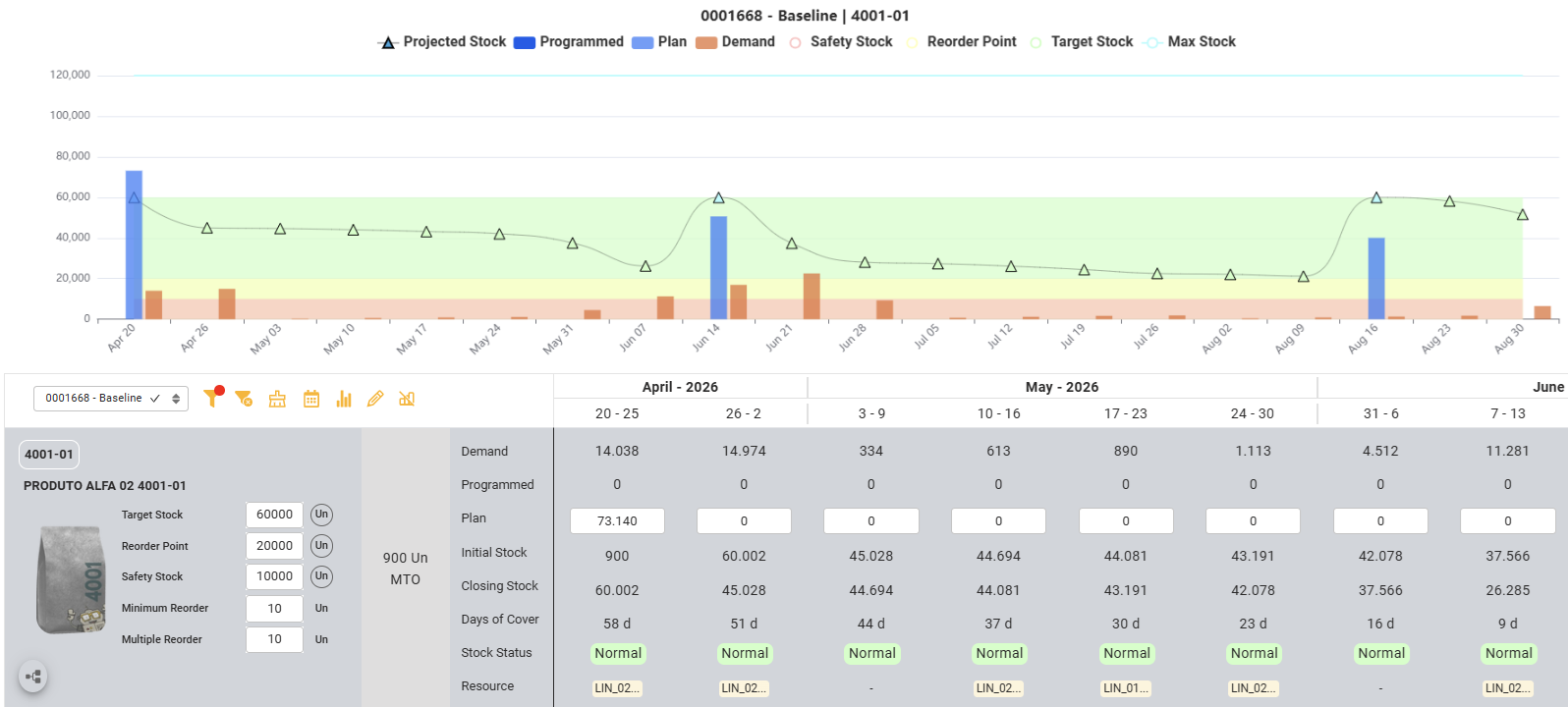
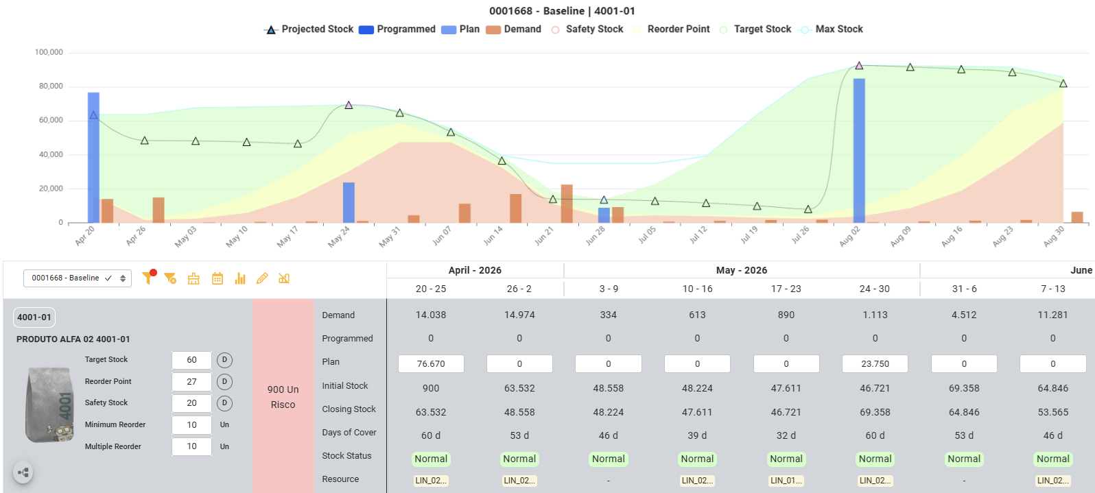
Target in Days vs. Units: Why Static Targets Fail
Once you have calculated your safety stock, the next decision is how to express your inventory target. Most planners default to units, keep 60,000 units of SKU X. This works in stable contexts, but breaks down the moment demand changes shape: seasonality, growth, promotions, product lifecycle. The alternative is to express the target in days of cover, which automatically scales with future demand.
Why this matters
- •A unit-based target gives you the same buffer regardless of where you are in the demand cycle, exactly when you need different protection.
- •A day-based target translates business intent (I want X weeks of safety) into a policy that adapts as the forecast evolves.
- •Communication across teams improves: We are carrying 32 days of cover is universally understood across functions. We are carrying 47,611 units is not.
Days of cover should be the default for any SKU with non-flat demand. Reserve unit-based targets for truly stable, low-volume items where conversion adds no value.
Common Inventory Management Mistakes
Even well-intentioned companies make recurring inventory management mistakes. Recognizing these patterns is the first step to correcting them.
Classifying ABC by volume only
Never do ABC by volume alone and never mix units of measure. An "A" item by volume may have very low margins, while a "B" item by volume might be the most profitable in the portfolio. Classification should consider financial value and impact on results.
Forgetting the Review Period in Lead Time
A common mistake is sizing safety stock against lead time alone, ignoring how often you actually review the replenishment policy. If your lead time is 5 days but you only review the order every 7 days, your real exposure window is 12 days — not 5. The review period acts as an extension of lead time: it expands the window during which you have no chance to react. In every safety stock formula, the lead time should be replaced by lead time + review period. Continuous-review policies are extremely rare in practice.
Confusing Variability with Forecast Error
Uncertainty is not demand standard deviation — it is the difficulty of getting the forecast right. Many planners use historical demand standard deviation (σ) as if it were the same thing as forecast error. They are not. Demand variability measures how demand swings around the mean. Forecast error measures how wrong your forecast was. A seasonal demand can have high standard deviation, but if the pattern is known, it is predictable — what matters is the ability to anticipate the behavior. A highly seasonal product can have huge variability but small forecast error if seasonality is well captured. Sizing safety stock with the wrong metric leads to excess and stockouts, usually both, on different SKUs.
Single service level target
Setting 95% or 99% for everything seems simple but is inefficient. High-turnover, high-margin products deserve maximum protection. Unpredictable, low-volume items operate better with lower targets, avoiding unnecessary stock accumulation.
Underestimating C items
CX has low impact and stable demand, accepting lower service levels with little safety stock. CZ is highly volatile and, despite seeming to need more protection, is usually the largest source of sleeping stock. In practice, setting lower targets for CZ avoids unnecessary accumulation.
Treating Lead Time as Fixed and Reliable
Most safety stock calculations assume lead times are stable and predictable. In reality, supplier lead times vary — sometimes dramatically. Worse: historical lead time variability is often a poor predictor of future variability, because the underlying causes (supplier capacity, logistics disruptions, geopolitical events) shift over time. Lead time uncertainty deserves explicit treatment in your policy, not a static average pulled from the ERP.
Setting Policy and Forgetting It
Inventory policy is not a project, it is a process. Demand patterns shift, suppliers change, products mature or decline, business strategy evolves. A policy calibrated 18 months ago is almost certainly miscalibrated today. Best-in-class teams review their ABC-XYZ classification and service level targets quarterly, not annually.
How We Solve It with NPLAN
NPLAN solves each of these challenges in an integrated and automated way, eliminating the operational complexity of maintaining a differentiated inventory policy.
Automatic and Always Updated Segmentation
The ABC-XYZ classification is automatically recalculated as demand and consumption data evolve. This eliminates the risk of obsolete classifications, one of the biggest problems for those doing manual segmentation in spreadsheets.
Strategies by Criticality Classification
Strategies can be segregated into different criticality classifications, with distinct policies for finished goods, intermediates, and raw materials. Additionally, exceptions can be defined for specific SKUs when needed.
Replenishment, Service Level, and Cycle by Segment
For each classification, NPLAN allows configuring the appropriate replenishment strategy, target service level, and ideal replenishment cycle, all differentiated and aligned with business drivers.
Forecast Quality Integration
NPLAN ties safety stock calculation directly to forecast accuracy at the SKU level. As your forecasting process matures, buffers automatically reduce, converting forecast quality improvements into cash freed from inventory, with measurable ROI.
Financial Integration
The impact of each policy is translated into tied-up capital, allowing inventory decisions to be evaluated from a financial perspective, not just operational.
Physical Occupancy Projection
Projected inventory from the policy is converted into physical storage space occupancy, anticipating capacity bottlenecks before they happen.
Stock Days Conversion
All projections are also presented in stock days, facilitating communication between areas and comparison across product categories.
Inventory Health Analysis
The defined policy is automatically compared with the current inventory situation, generating a health analysis that identifies excesses, stockouts, and deviations. A topic we'll explore further in an upcoming article.
Scenario Simulation
Everything can and should be simulated with different strategies through scenario comparison. NPLAN allows evaluating the impact of policy changes before implementing them, reducing risk and accelerating decisions.
The image below illustrates how NPLAN presents the inventory policy in a consolidated view: each SKU is automatically classified in the ABC-XYZ matrix, with replenishment strategy, service level, cycle, and safety stock calculated and displayed in a single integrated view, including impacts on tied-up capital and storage occupancy.
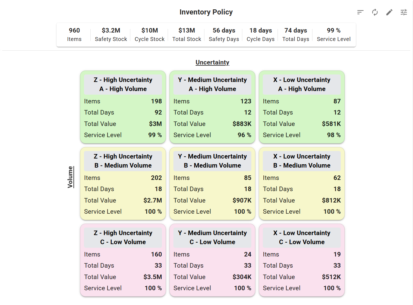
With NPLAN, inventory policy goes from being a static exercise in spreadsheets to a living, integrated, and strategic process, always aligned with business reality.
10 Tips & Tricks to Reduce Stock Today
Beyond calibrating policy, here are 10 levers you can pull this quarter to free up working capital. Each item has a different effort/impact profile, start with the Quick Wins.
Kill Obsolete Stock
Map items with no turnover for extended periods and define an immediate action plan.
Flag Slow Movers
Items with very low turnover consuming space and capital unnecessarily.
Cancel Open Orders
Review pending purchase orders for items with excess or downward-revised demand.
Negotiate Supplier Returns
Negotiate return of materials still within contractual terms and conditions.
Run Targeted Promotions
Use campaigns to accelerate turnover of excess items, especially CY and CZ.
Pause New Launches
Reassess planned launches when the portfolio already shows excess in the same category.
Donate or Dispose
Last resort for irrecoverable items. Frees space and reduces carrying costs.
Recalibrate Replenishment Parameters
Adjust minimum lots, lead times, and reorder points based on actual consumption and supply data.
Sync Policy with Commercial Strategy
Ensure service level targets reflect business priorities, not just generic standards.
Monitor Continuously with Real-Time Indicators
Continuous monitoring with coverage, turnover, and aging indicators to act before the problem grows.
The combination of differentiated policy with active management of existing inventory is what separates companies with well-sized stock from those that just "push" excess to the next cycle. NPLAN allows configuring these policies by segment and tracking adherence with real-time coverage, turnover, and aging indicators.
Policy Is a Wish — Reality Has Constraints
Everything we've discussed so far — ABC-XYZ segmentation, safety stock formulas, days of cover, differentiated service levels — produces what the business wishes to hold in inventory. It's the ideal policy: mathematically sound, segmented by criticality, calibrated to forecast quality. But the calculated policy is not yet an executable plan. Between the wish and the reality sits a layer of constraints that can make even the most carefully designed policy impossible to follow as-is.
The Constraints That Reshape Your Policy
Four families of constraints typically force the calculated policy to bend:
Physical Storage
You can calculate that SKU X needs 60 days of cover, but if your warehouse can't physically hold that volume, the policy is fiction. Storage capacity — pallets, shelves, refrigerated space, hazmat areas — is a hard ceiling. Inventory policy must be validated against physical occupancy, not just financial logic.
Working Capital
The ideal policy might require $15M in inventory. The business may only have $9M available. Capital constraints don't disappear because the formula says otherwise — they force prioritization: which segments get the full buffer, which get partial, which run lean and accept higher stockout risk.
Lot Sizes and MOQs
Safety stock might be 200 units, but if the supplier's minimum order quantity is 5,000 — or your production batch size is 10,000 — the actual replenishment will be driven by the lot, not by the safety stock. The policy says "carry 200"; reality delivers 5,000 every time you reorder. Lot size often overrides policy in practice.
Production Capacity
Even if every other constraint is satisfied, you can only build what your factory can produce. As covered in our Capacity & Orders article, capacity isn't just machine hours — it's tooling, labor polyvalence, warehousing buffer between operations, setup time, and preventive maintenance. A policy that requires 240 hours of production per week from a center with 160 hours of capacity is mathematically valid and operationally impossible.
Why Your Policy Should Vary Over Time
A second insight follows from the constraints above: the same SKU may justify different policies at different times of the year. Inventory policy is often presented as a static target — "30 days of cover" or "X units of safety stock." But the realities that drive policy are anything but static.
Three common scenarios where a period-aware policy outperforms a static one:
Anticipating Planned Shutdowns
Collective vacations, factory holidays, planned maintenance windows. If production stops for two weeks in July, the policy needs to ramp up cover in June — temporarily exceeding the "ideal" steady-state target — to avoid stockouts during the shutdown. After the shutdown, cover returns to baseline.
Leveling Capacity Ahead of Peaks
When a high season is coming and capacity is tight, building inventory ahead of the peak smooths the production load. This requires the policy to temporarily increase target stock weeks before demand spikes — converting future capacity stress into present inventory. Without this, peak season either misses sales or creates costly overtime/outsourcing.
Phasing Down Before Product Transitions
When a SKU is being discontinued or replaced, the policy should phase down well before the cutover — reducing target stock progressively to avoid leftover inventory of obsolete material. A static policy keeps building stock right up to the discontinuation date.
The takeaway: calculating the right policy is necessary but not sufficient. The policy is the wish. The plan is what survives contact with constraints.
This is why inventory policy doesn't live in isolation. It feeds into supply planning — where lot sizes, lead times, and material availability shape what can actually be replenished — and into capacity planning, where production constraints, shared resources, and calendars determine what can actually be built.
See how this plays out end-to-end in our companion articles:
Supply Planning: from static MRP to dynamic plan
How the calculated policy becomes an executable replenishment plan, respecting lot sizes, lead times, and supplier calendars.
Read article →Capacity & Orders: finite scheduling and end-to-end synchronization
How production capacity, tooling, labor, and maintenance reshape the plan that policy alone cannot deliver.
Read article →Inventory policy answers "what should I hold?". Supply planning answers "what can I get?". Capacity planning answers "what can I build?". A mature S&OP process keeps these three questions in sync — because optimizing one in isolation guarantees the other two will break.
What This Article Didn't Cover
This article covered inventory policy with focus on finished goods and independent demand, with extensions for raw materials and supply variability. Two important topics fell outside the scope and deserve mention:
Multi-echelon. The entire discussion above is single-echelon: one SKU, one stocking point, one buffer. Real supply chains often have multiple stocking points (factory → central DC → regional DCs → store), and safety stock at each level interacts in non-obvious ways. The operational question "in which echelon do I place the buffer" significantly changes the recommendations in this article. It's a distinct optimization problem with its own literature.
DDMRP (Demand Driven MRP). An alternative paradigm that places buffers at strategic decoupling points in the chain, rather than spreading safety stock across every SKU at every level. It uses buffer zone logic (green/yellow/red) and dynamic adjustment based on average daily usage (ADU). It's seen growing adoption in complex BOM manufacturing and multi-stage production, and is worth knowing even for those choosing the traditional paradigm covered in this article.
Both topics are candidates for dedicated articles continuing this series.
Test Your Knowledge
Assess whether you've mastered differentiated inventory policy concepts with this quick quiz.
Two SKUs have the same demand variability. SKU A has 5% forecast error; SKU B has 30% forecast error. Which one needs more safety stock?
Inventory policy is not about having more or less. It's about having the right stock, in the right segment, with the right target. ABC-XYZ segmentation, combined with the seven service level drivers, transforms inventory from a cost center into a competitive advantage.
Looking for a local partner specialized in Supply Chain Planning Implementation?
Next in the series: Supply Planning
Inventory policy is only the starting point. See how NPLAN turns policy into supply orders that respect capacity, lot sizes and supplier windows.
Read the next article